Imagine you’re analyzing a company’s sales data. You have a sale date, a delivery date, and an invoice date. You want to compare trends based on when sales occurred versus when orders were delivered, and you need filters and aggregations for both. What’s the best way to model this?
The Problem with a Single Calendar Table for Multiple Dates
Power BI modeling best practices often recommend using a single calendar table when dealing with fact tables that contain multiple date columns. In such cases, we typically define an active relationship with one date column (e.g., Sales[Sale Date]) and inactive relationships with the others (e.g., Sales[Delivery Date]).
To work with these inactive relationships, we use the USERELATIONSHIP() function inside CALCULATE() to switch the active date context dynamically. This is a well-established approach, but as we’ll see, it introduces several limitations that impact flexibility, usability, and maintainability.
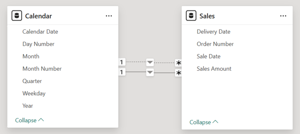
Consider this simple model, where the active relationship is based on Sales[Sale Date], and an inactive relationship exists between Sales[Delivery Date] and the Calendar table:
Let’s say we wanted to aggregate Sales Amount over Sale Date. We could quite simply define this measure:
Total Sales = SUM ( Sales[Sales Amount] )
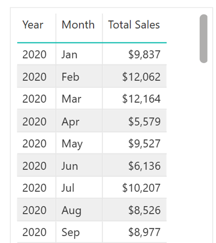
Since the default active relationship is with Sales[Sale Date], we can now display total sales by sale date in a visual without any extra effort:

However, what if we wanted to aggregate Sales Amount over Delivery Date? We would need a second measure to override the active relationship between the two tables and instead activate the one on Delivery Date:
CALCULATE (
SUM ( Sales[Sales Amount] ),
USERELATIONSHIP ( Sales[Delivery Date], Calendar[Calendar Date] )
)
If we wanted to perform other aggregations, such as the sum of order quantities, we would find ourselves creating similar pairs of measures, one over the default relationship and another over the inactive relationship over Delivery Date.
Second Challenge: Displaying Multiple Date Attributes in Tables
Another challenge arises when trying to display date-related attributes for both Sale Date and Delivery Date in a table visual.
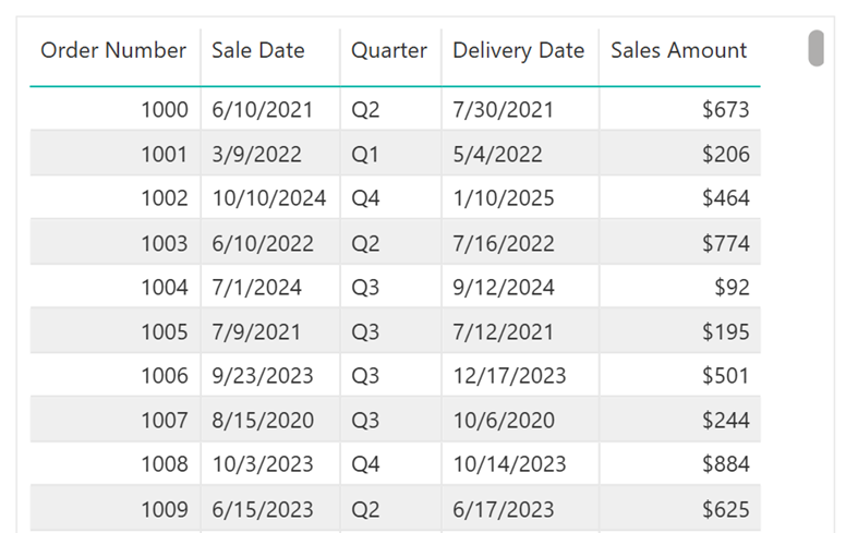
At first, it is quite simple: just use columns from the Sales table:
However, what if we are asked to include the quarter of both dates? We could do it for Sales Date by dragging the Quarter column from the calendar table because of the active relationship:
However, for Sales[Delivery Date], Power BI cannot retrieve its corresponding quarter directly because there is no active relationship between the calendar table and Delivery Date.
To resolve this, we would need calculated columns or measures, adding unnecessary complexity:
Delivery Quarter =
CALCULATE (
SELECTEDVALUE ( Calendar[Quarter] ),
USERELATIONSHIP ( Sales[Delivery Date], Calendar[Calendar Date] )
)
For a simple requirement like showing the quarter, this level of extra work is unnerving.
Third Challenge: Filtering and Slicing by Multiple Dates
Filtering by both Sale Date and Delivery Date also becomes problematic. It is not possible to add a slicer by the year or by the weekday of delivery dates, for example, because the relationship is inactive. The slicer would have no effect on the other visuals.
A Better Approach: Using Multiple Calendar Tables
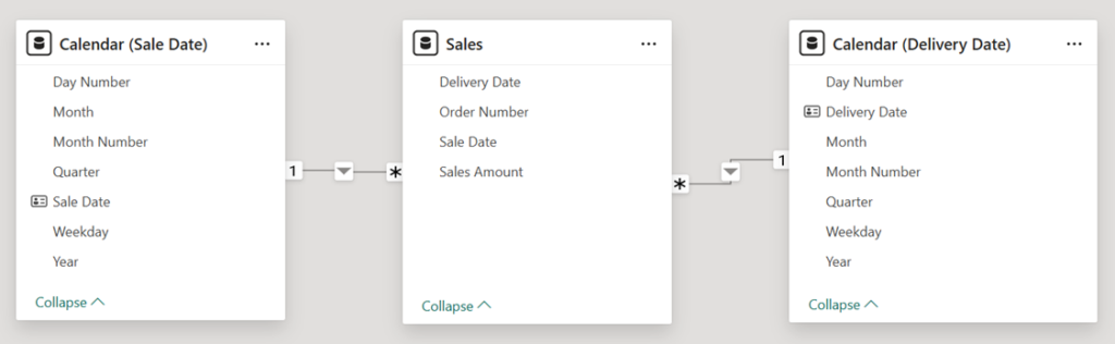
Instead of relying on a single calendar table with multiple relationships, we can create separate calendar tables, each linked by an active relationship to a corresponding column in the fact table.
With this model:
- One measure suffices for all date contexts (no need for duplicate CALCULATE() measures).
- Date attributes (quarters, weekdays, fiscal years) are easily accessible for both dates.
- Slicers can filter by Sale Date and Delivery Date independently.
To avoid confusion, it is good practice to name these tables clearly, e.g., Calendar (Sale Date) and Calendar (Delivery Date). Also, note that the column Calendar Date in the original table has been renamed in the two copies. This is also very convenient (and helps minimize errors) when configuring visuals.
Only One Measure for Sales Amounts
Now our original, simple measure:
Total Sales = SUM ( Sales[Sales Amount] )
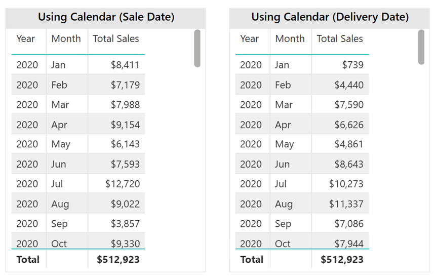
Works seamlessly across both date contexts, without needing modifications. Here we use it on both visuals:
An Aside
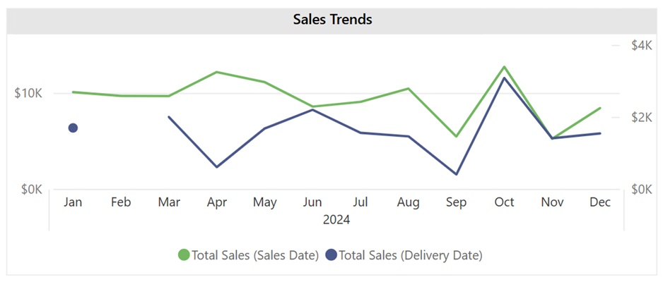
There’s one scenario where multiple date tables require extra work: plotting sales amounts by both Sale Date and Delivery Date on the same time axis. Suppose we want a line chart with Year/Month on the X axis and two lines, one for sales amount based on Sale Date and another for sales amount based on Delivery Date.
Now assume we decide to use Calendar[Sale Date] for the X axis. If we add the Total Sales Amount measure for one of the lines, we would see amounts by sale date, as expected.
What about sales by delivery date? We would need a second measure to map the X axis values to delivery dates. This would be an additional measure like the one required with the one-calendar-table model. For the current model, this may be achieved by using TREATAS():
Total Sales (Delivery Date) =
CALCULATE (
[Total Sales],
TREATAS (
VALUES ( ‘Calendar (Sale Date)'[Sale Date] ),
‘Calendar (Delivery Date)'[Delivery Date]
)
)
Here’s the chart with both measures (we renamed Total Sales to Total Sales (Sales Amount) in the chart):
Exercise for the reader: The chart ends in December 2024, the last month with sales. But there are deliveries in 2025. How to extend the X axis to show those delivery months?
Better Table Visuals
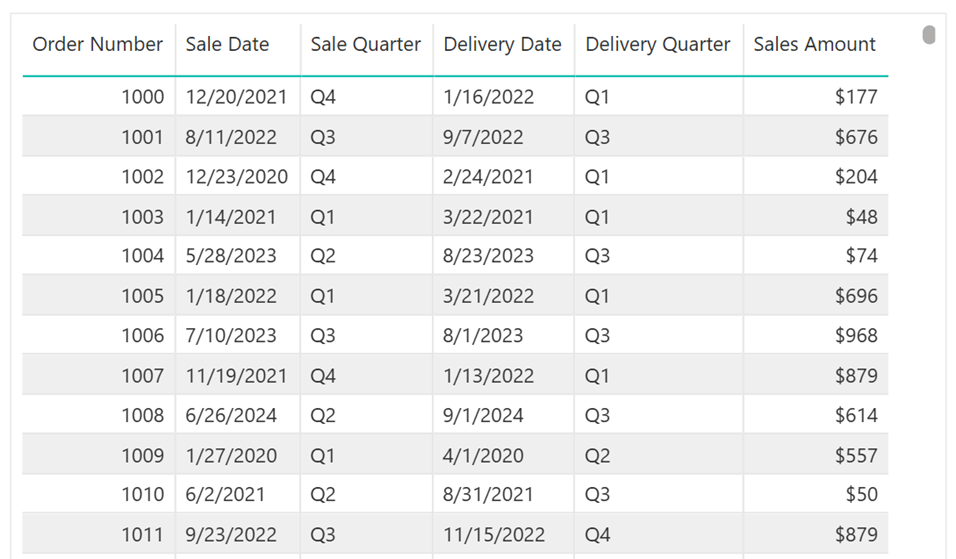
We can now create a single table visual with attributes about both dates by just dragging the corresponding columns from the three tables with no need for fancy workarounds:
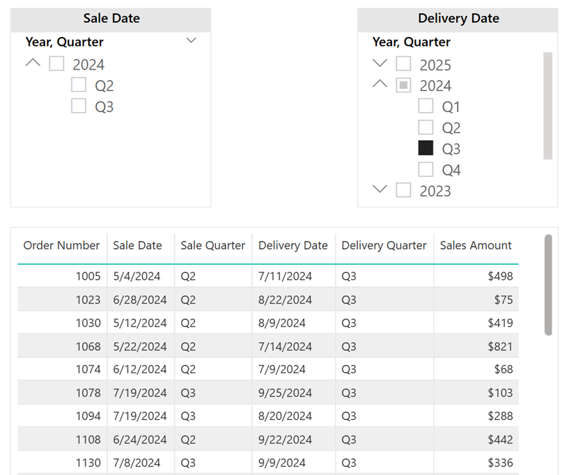
Better Slicers
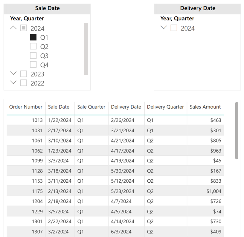
Filtering by Sale Date and Delivery Date now works natively. In the following images, each slicer filters its respective date column without needing any workarounds:
When Should You Stick to One Dates Table?
While multiple date tables offer significant flexibility, there may be one or more reasons for which a single calendar table may still be preferable:
- Large models – Too many date tables can increase model size and refresh times.
- Too many date columns – If a fact table has five or more date columns, separate tables could become excessive.
- Complex time intelligence needs – If you need to compare cumulative trends across multiple dates (e.g., YTD sales by order date vs. YTD shipments by delivery date), USERELATIONSHIP() may be easier.
Common Mistakes to Avoid When Using Multiple Date Tables
This approach also has its pitfalls, to note:
- Accidentally filtering the wrong date table (minimize this by using clear table and column names).
- Forgetting to mark each date table as a “date table” (required for convenience when using built-in time intelligence functions).
Final Thoughts
For many reporting needs, using multiple date tables is a more scalable and intuitive approach than relying on USERELATIONSHIP(). It simplifies calculations, improves usability, and makes reports easier to maintain.
If you’ve been struggling with complex measures to handle multiple dates, consider restructuring your model—you might find it makes reporting far more flexible with much less effort.